For this part, I ended up training a denoising neural network. I display results in the next couple parts as requested.
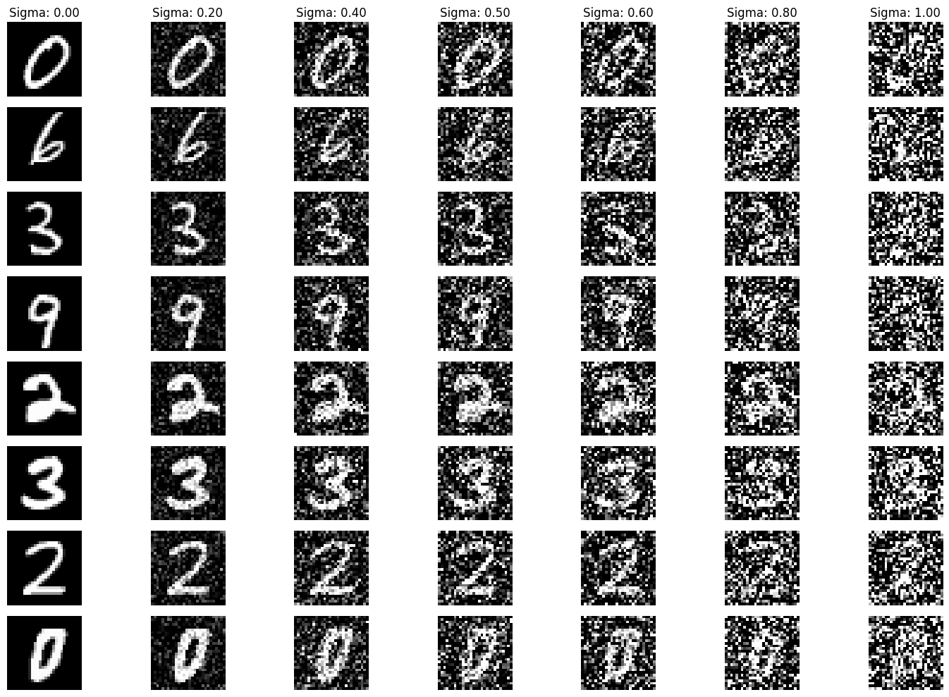
Listed below is a visualization showing how a higher sigma visually affects the images

|
The denoising UNet was trained for 5 epochs, with a hidden dimension D of 128 and sigma = 0.5.
|
Results after epoch 1 completed 
|
|
Results after epoch 5 is completed 
|
|
Final Training Loss vs Step curve 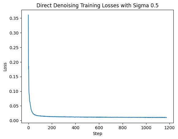
|
Results shown for sigma values 0, 0.2, 0.4, 0.5, 0.6, 0.8, and 1.0 are shown below
|
Sigma = 0 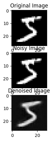
|
Sigma = 0.2 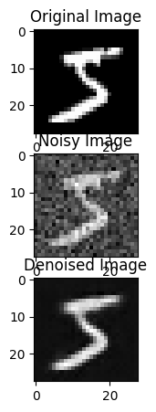
|
Sigma = 0.4 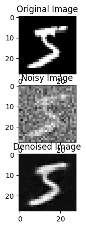
|
Sigma = 0.5 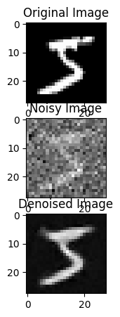
|
Sigma = 0.6 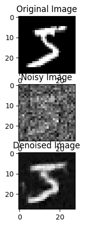
|
Sigma = 0.8 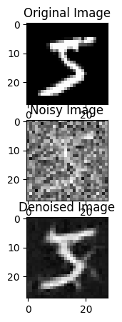
|
Sigma = 1.0 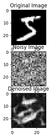
|
Below, you will find training loss curves from a 5 epoch and 20 epoch run. You will also find examples of denoising attempts from batch data provided during train time, and some examples of sampling the model from scratch.
|
Visualization of data on the 5th epoch 
|
|
Training run loss curve 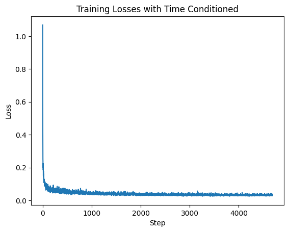
|
|
Visualization of data denoised during on the 5th epoch 
|
|
Visualization of data sampled from scratch during on the 5th epoch 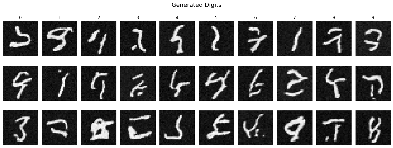
|
|
Visualization of data denoised on the 20th epoch 
|
|
Visualization of data sampled from scratch during on the 20th epoch 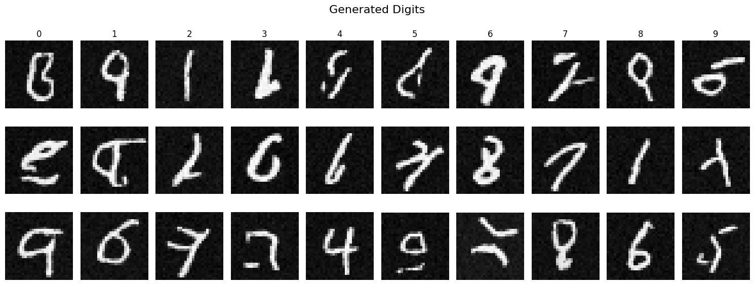
|
|
Training run loss curve 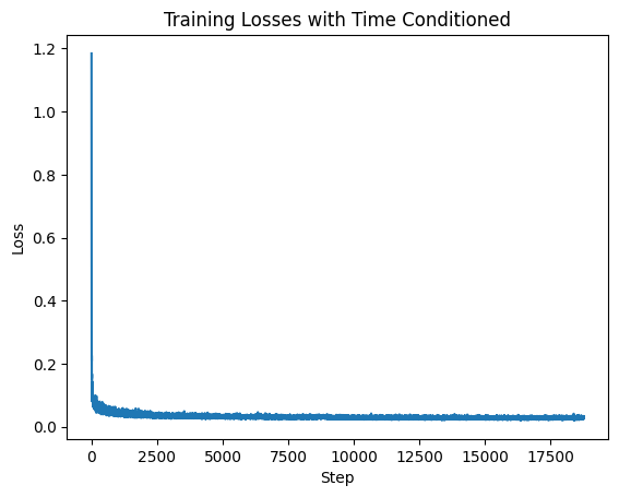
|
The denoising UNet was trained for 5 epochs, and 20 epochs with a hidden dimension D of 128. Notably for the sake of performance, I enabled the training to sample batches of timesteps rather than one single timestep for all.
Previously, I had faced accuracy limitations, where my mean squared loss for optimization would taper off around 0.4. One notable suggestion during office hours was to replace the last "Conv" layer with a Conv(3, 1, 1), or a convolution layer with a kernel size of 3, and padding & stride of 1.
But we're here now. In 2.4, I implemented class conditioning for my already time conditioned diffusion model. Below, you will find training and sampling results from a run consisting of 5 epochs, and then 20 epochs. Each run lists the training loss curve (training requirements), alongside visualizations of the training data being fed to the class conditioning model and the output. At epoch 5 and 20, I also sample the model (completely from scratch - passing in a random tensor), and show how the digits are being listed.
|
Visualization of data on the 5th epoch 
|
|
Visualization of data generated after the end of the 5th epoch 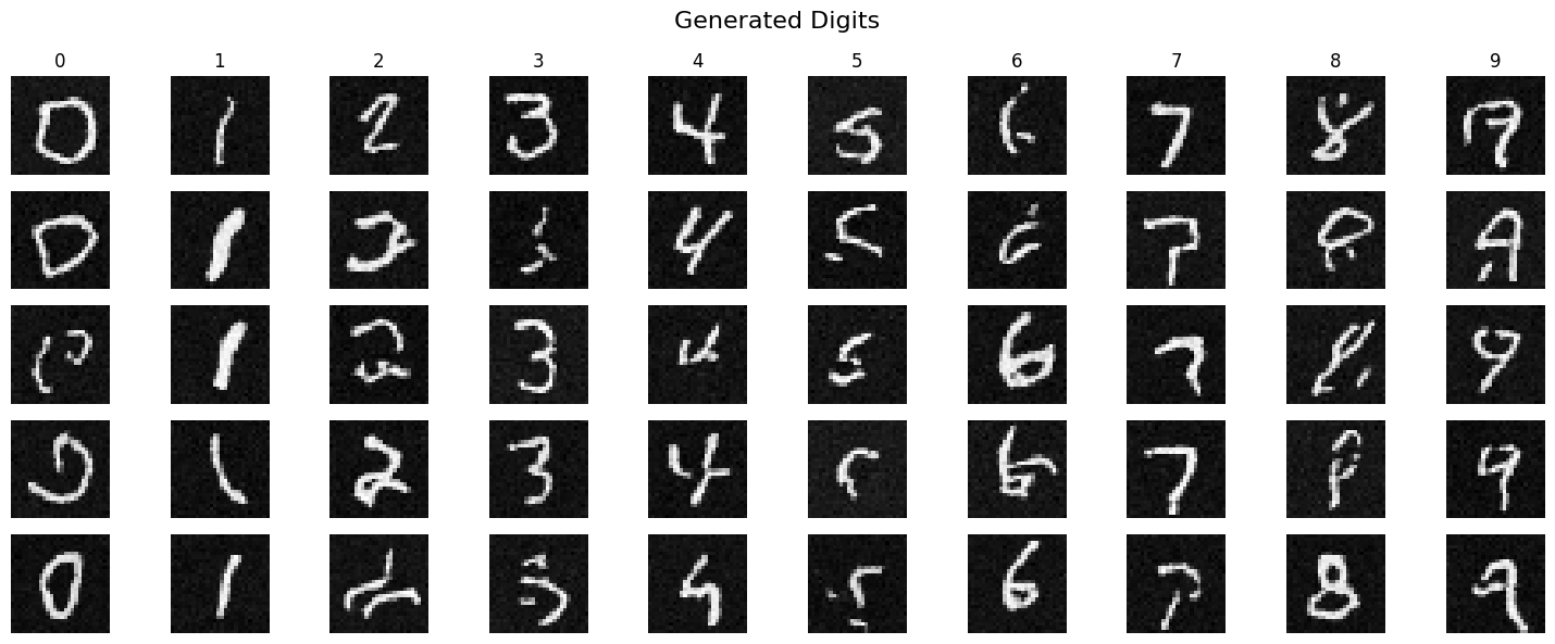
|
|
Training run loss curve 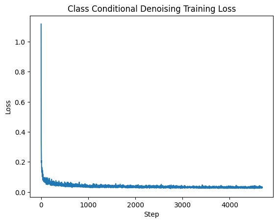
|
|
Visualization of data denoised during on the 5th epoch 
|
|
Visualization of data sampled from scratch during on the 5th epoch 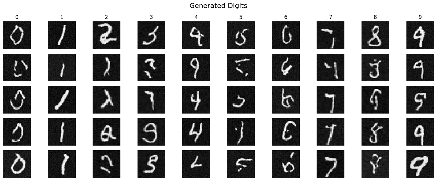
|
|
Visualization of data denoised on the 20th epoch 
|
|
Visualization of data sampled from scratch during on the 20th epoch 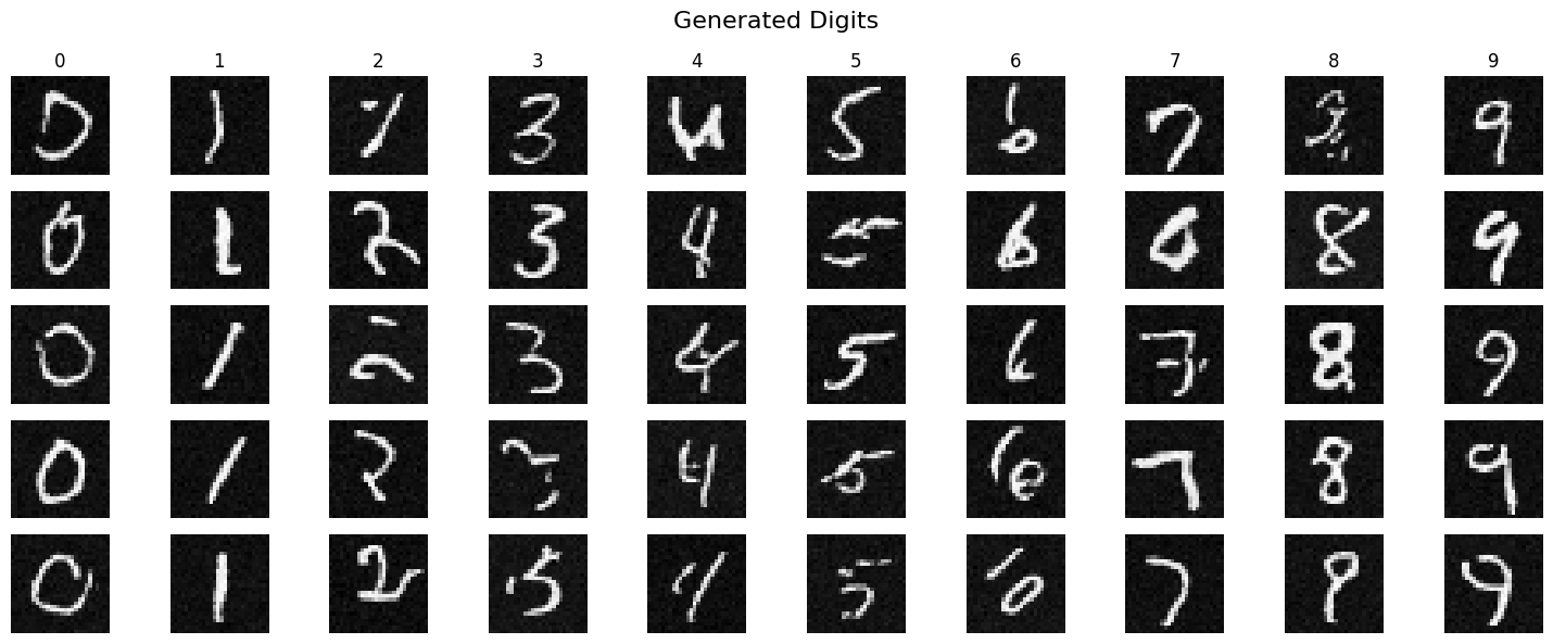
|
|
Training run loss curve 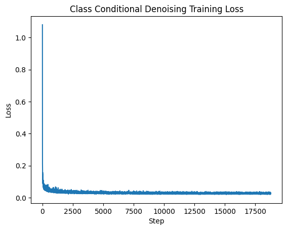
|