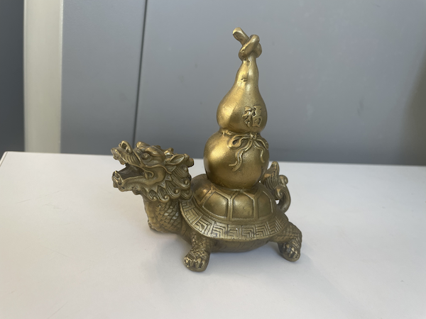
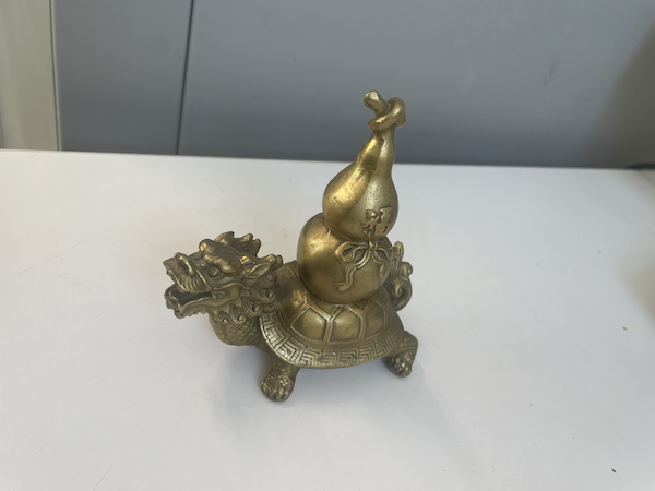
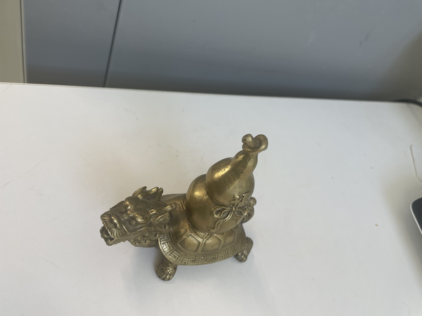
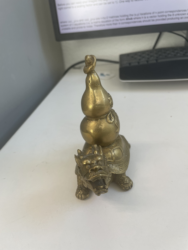
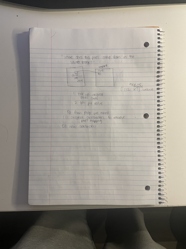
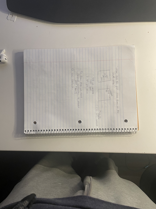
First, a bit of a repeat from part A ... if you're making a beeline for the automatically generated images, scroll down to the bottom, Part 6! (CTRL + F "Part 6")

|

|

|

|

|

|
        def computeH(pts_src, pts_dest):
            A = []
            for (x_s, y_s), (x_d, y_d) in zip(pts_src, pts_dest):
                A.append([x_s, y_s, 1, 0, 0, 0, -x_d * x_s, -x_d * y_s])
                A.append([0, 0, 0, x_s, y_s, 1, -y_d * x_s, -y_d * y_s])

            # Convert to numpy linear equation
            A = np.array(A)
            b = pts_dest.reshape(-1, 1)

            H = (np.linalg.pinv(A.T @ A) @ A.T @ b)
            return np.vstack((H, 1)).reshape(3, 3)
        def warpImage(im, im_pts, H, output_shape=None):
            h, w = im.shape[:2]
            corners = np.array([[0, 0], [w-1, 0], [w-1, h-1], [0, h-1]])
            ones = np.ones((4, 1))
            corners_h = np.hstack([corners, ones])

            warped_corners = (H @ corners_h.T).T
            warped_corners /= warped_corners[:, [2]]  # Normalize by z

            min_x, min_y = np.min(warped_corners[:, :2], axis=0)
            max_x, max_y = np.max(warped_corners[:, :2], axis=0)

            if output_shape is None:
                output_shape = (int(np.ceil(max_y - min_y)), int(np.ceil(max_x - min_x)))

            xx, yy = np.meshgrid(np.arange(-output_shape[1], output_shape[1]), np.arange(-output_shape[0], output_shape[0]))
            xx_out, yy_out = np.meshgrid(np.arange(0, output_shape[1]), np.arange(0, output_shape[0]))

            out_homog_coords = np.stack([xx.ravel(), yy.ravel(), np.ones_like(xx).ravel()], axis=1)
            translation_matrix = np.array([[1, 0, -min_x],
                                        [0, 1, -min_y],
                                        [0, 0, 1]])
            H_inv = np.linalg.inv(translation_matrix @ H)


            mapped_coords = (H_inv @ out_homog_coords.T).T

            mapped_coords /= mapped_coords[:, [2]]  # Normalize by z
            x_mapped = mapped_coords[:, 0]
            y_mapped = mapped_coords[:, 1]

            new_coords_x = xx.ravel()
            new_coords_y = yy.ravel()

            valid_mask = (x_mapped >= 0) & (x_mapped < w) & (y_mapped >= 0) & (y_mapped < h)

            im_warped = np.zeros((output_shape[0], output_shape[1], im.shape[2]), dtype=im.dtype)  # Create blank output
            for i in range(im.shape[2]):  # Interpolate each channel
                im_warped_channel = scipy.interpolate.griddata(
                    (new_coords_y[valid_mask], new_coords_x[valid_mask]),  # input coordinates (valid only)
                    im[y_mapped[valid_mask].astype(int), x_mapped[valid_mask].astype(int), i],  # input values
                    (yy_out, xx_out),                                      # output grid
                    method='linear',
                    fill_value=0                                   # Fill out-of-bound pixels with 0
                )

                im_warped[:, :, i] = im_warped_channel


            orig_points_homogeneous = np.hstack((im_pts, np.ones((im_pts.shape[0], 1))))

            transformed_points = ((translation_matrix @ H) @ orig_points_homogeneous.T).T

            transformed_points /= transformed_points[:, 2].reshape(-1, 1)  # Normalize to get (x, y)

            return im_warped, translation_matrix, transformed_points[:, :2]
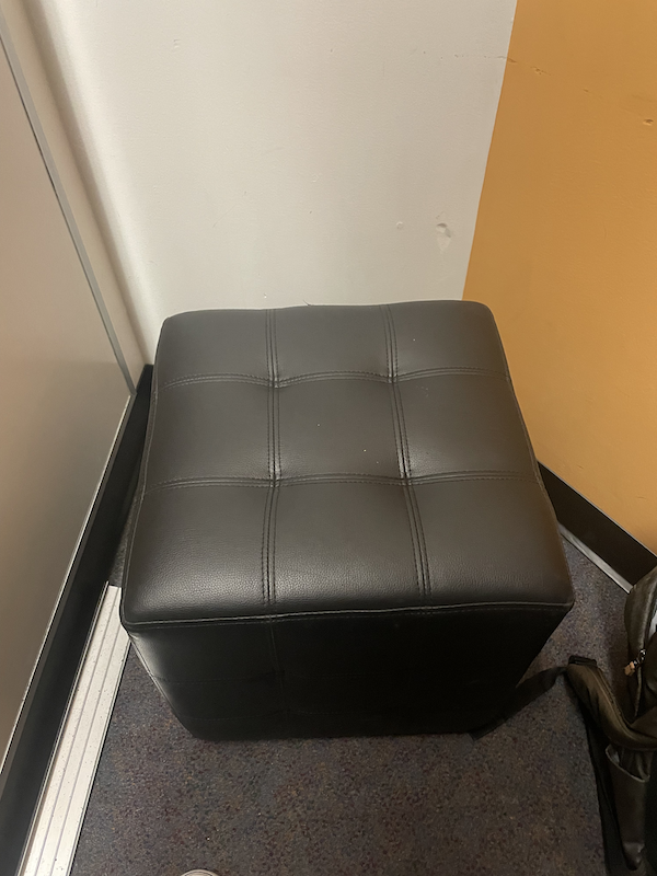
Original |
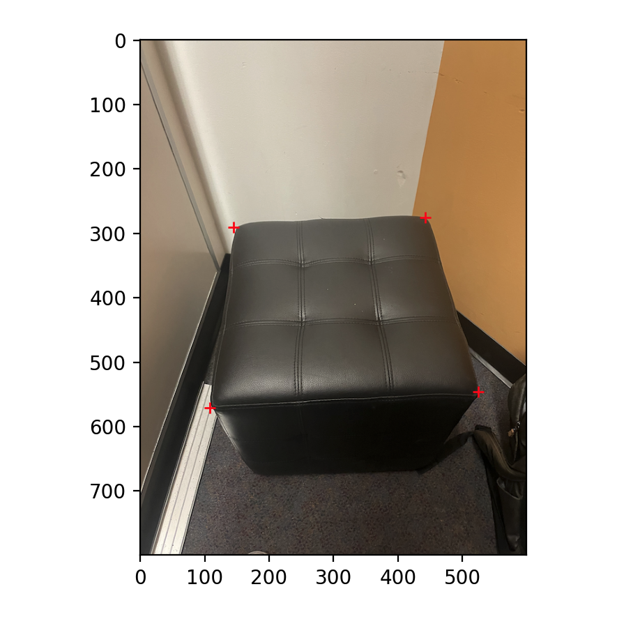
Labeled |
Rectified |

An Interesting Rectification (Original) |
Perspective Warp |
Perspective Warp |

An Interesting Rectification (Original) |
Perspective Warp |
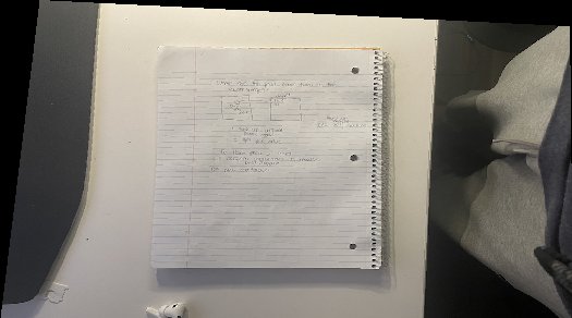
Perspective Warp |
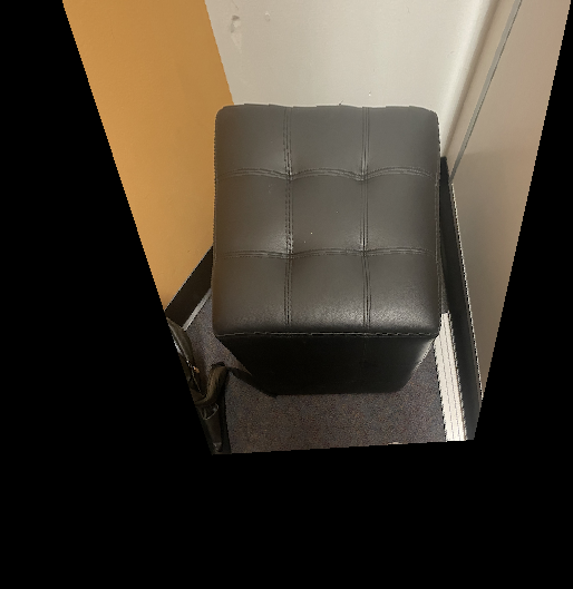
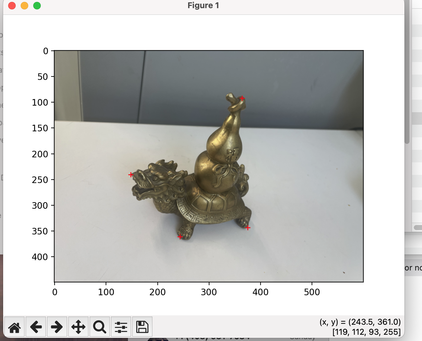
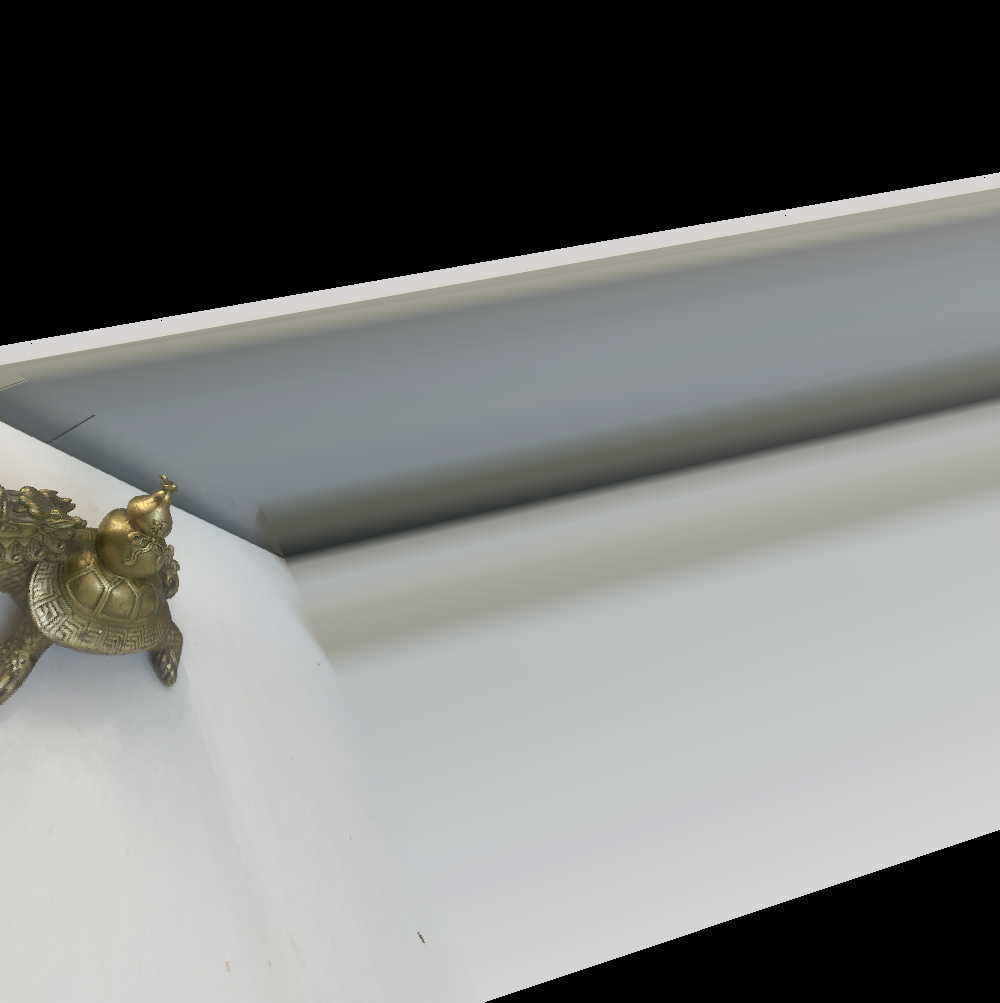
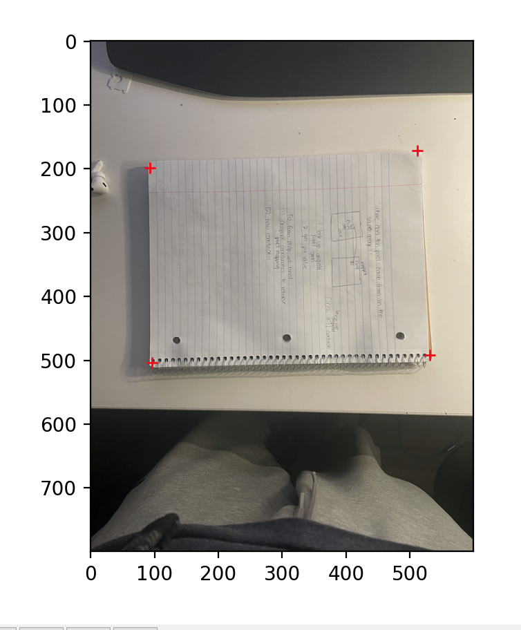
Check out the FIRST for the most "square"-ish object. All images were warped to the same four key points - [[100, 200], [300, 200], [300, 400], [100, 400]]. The rectified image wasn't initially looking like this. The changes I needed to make were to (1) rotate the image, and then (2) crop it down to remove excess black.
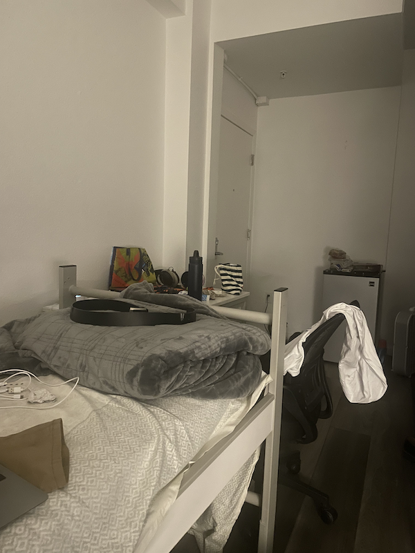
Image 1 |
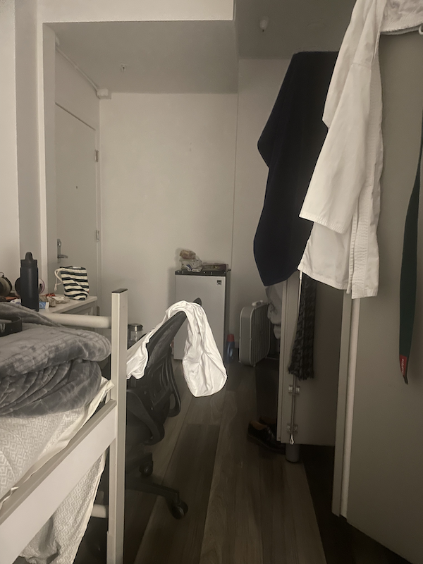
Image 2 |
Mosaic |
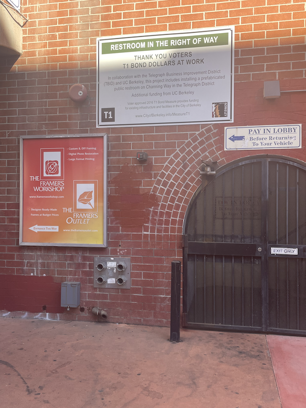
Image 1 |
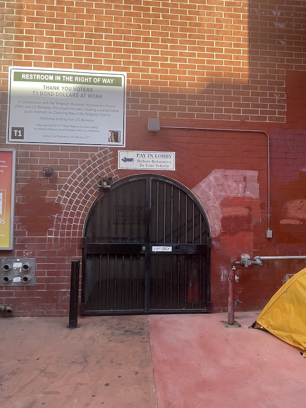
Image 2 |
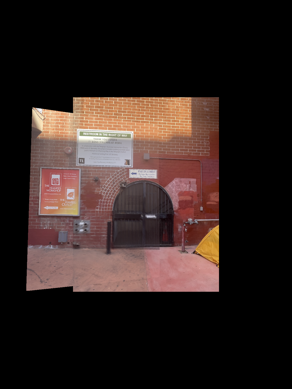
Mosaic |
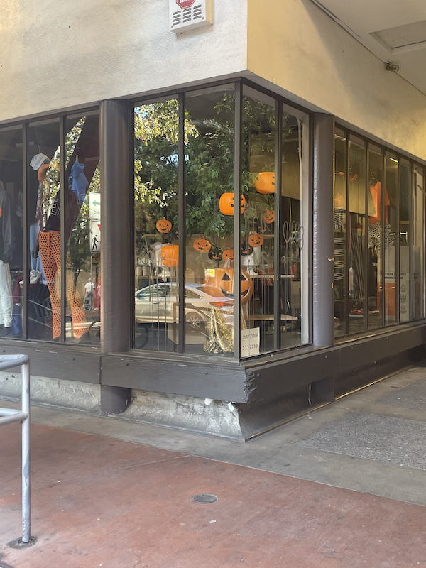
Image 1 |
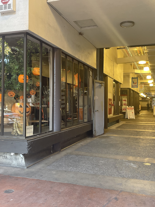
Image 2 |
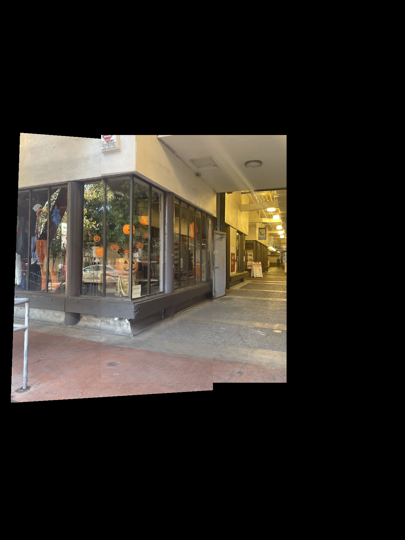
Mosaic |
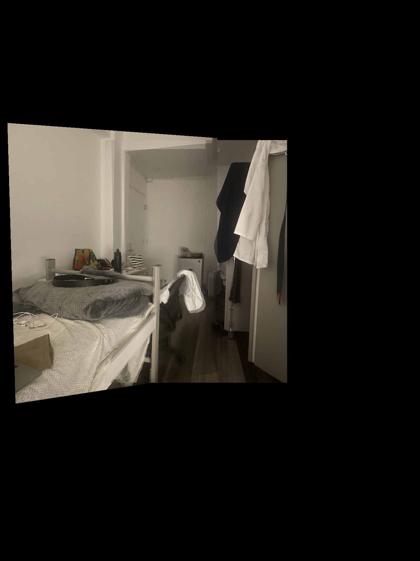
Learnings: Sometimes, sticking to the simplest method is the easiest. The mosaics took an extremely long time, as I tried to find extremely elaborate ways of improving image quality. Little did I realize that simply doing a weighted average over the intersection would suffice to provide the biggest jump in performance. Don't oversolve a problem unless required.
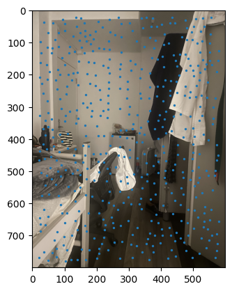
ANMS output between images. |
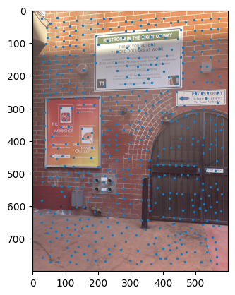
ANMS output between images. |
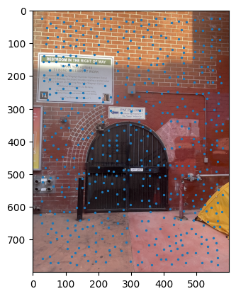
ANMS output between images. |
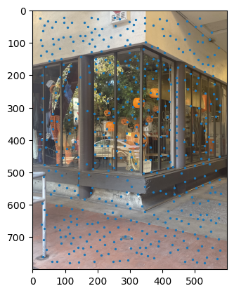
ANMS output between images. |
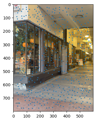
ANMS output between images. |
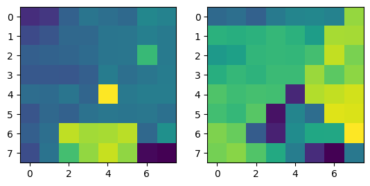
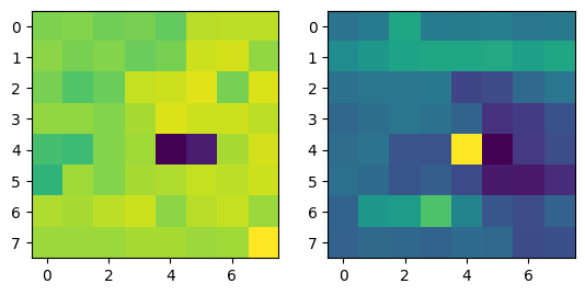
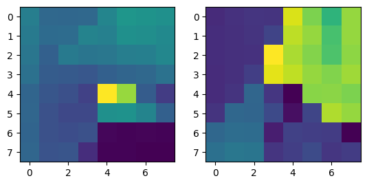
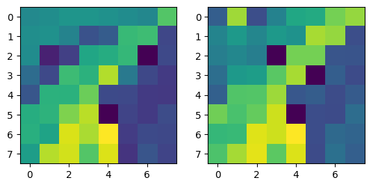
Notes: When I implemented the Harris algorithm, I initially was confused to why ANMS would be so crucial. However, that doubt was quickly cleared after seeing the results. I initially faced some challenges in verifying my output for ANMS was coming out right, especially given the large number of points - for the images you see, there are 500 points being created, with an edge supression of 20. I'm honestly still very dubious on whether modifying the edge score has a major impact in the process, changes in the value didn't seem to translate to understandable changes in output.
I still don't have much clarity on whether c_robust provides much value apart from more low level control to the ANMS algorithm. I didn't find much of a jump between c_robus = 0.9 and c_robust = 1. Perhaps in a high volume, low radius use case for feature control, but not very apparent here.
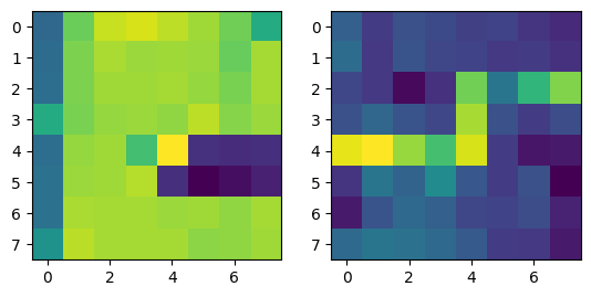
|
|
|
|
|
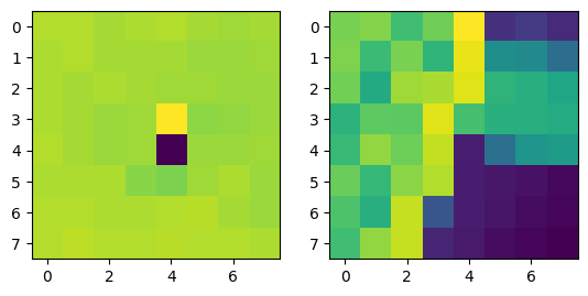
|
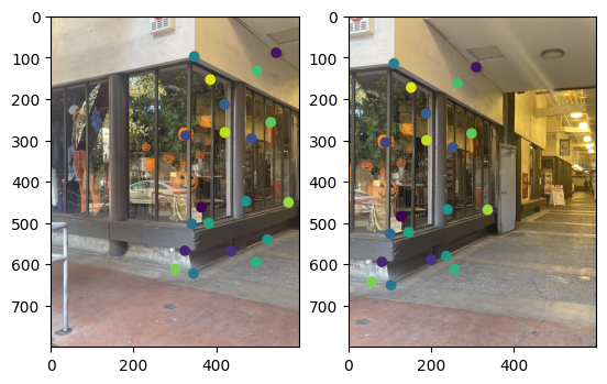
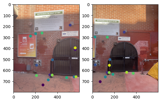
Here, I've dropped some features from the three mosaic images I've compiled. In my feature extraction algorithm, I only considered a single channel versus doing a grayscale or using all three channels. I intended to explore this, and discovered that some of my office hour peers who did end up implementing it with RGB (and with a blur, in some cases), didn't have much of a difference in results.
Note that two points from different images with the same color refer to corresponding points.
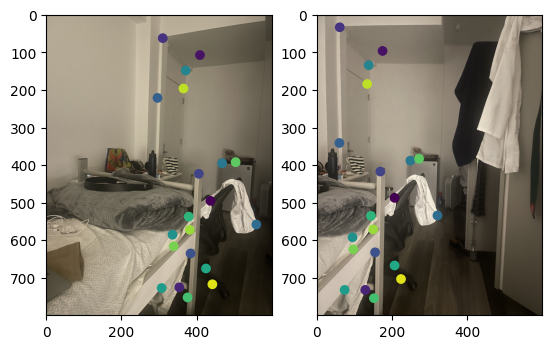
Correspondences between the two images in the room. |
|
|
|
Feature matching was more brutally challenging in finding the right parameters to even verify that the feature rejection algorithm was working. I found on Stack Overflow to use a Lowe's test ratio of around 0.8, but previous tests with 0.9 and 0.5 proved how differently accurate the results are when playing around with the rejection algorithm. I would say this "part of the pipeline" is easily the most relevant place to tune out of everything else.
Automated evaluation results.
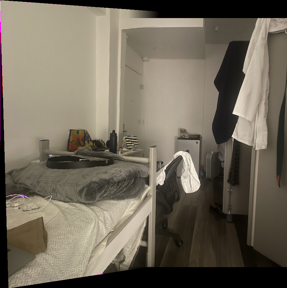
Manual Annotation |
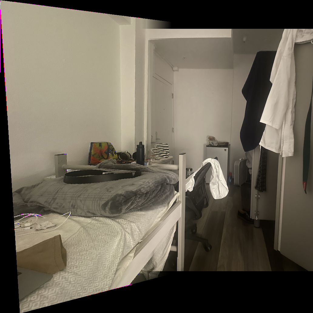
Automatic Annotation |
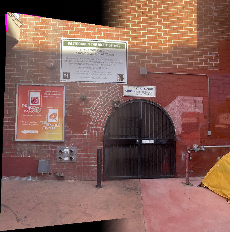
Manual Annotation |
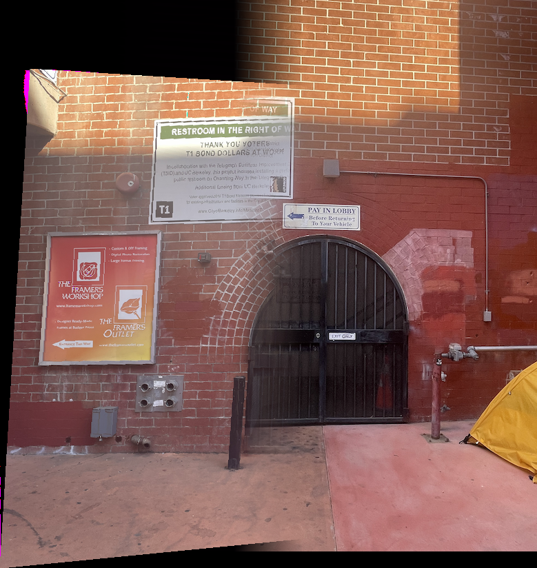
Automatic Annotation |
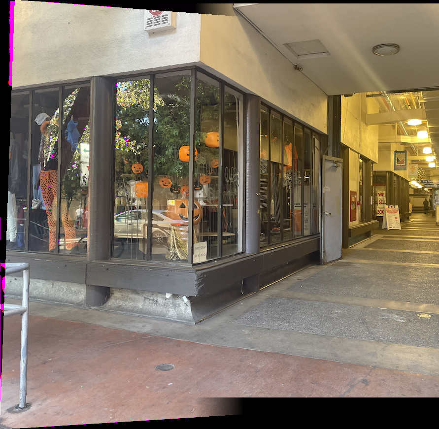
Manual Annotation |
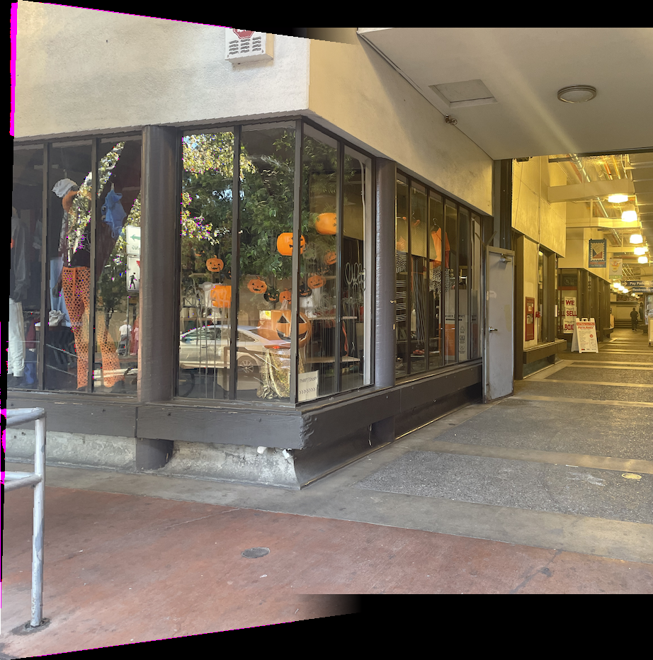
Automatic Annotation |
In many of the images I ran (but didn't show, for the sake of not pelting you with Mosaics), there was fair evidence to suggest that the automated algorithm provided similar output image wise to the manual stitching. Does that mean that homography, in it's infinite wisdom, is really a path to eyes, and thus the soul? I'll let you judge that. However, I did want to address the defects in the second image.
I've released the output from the automatically generated and manual homography matrices, and you'll see that they are, in areas that aren't infinitesimily small, often pretty close. In the actual image output, I noticed that the correspondences for the auto evaluation were all clumped together. I wonder if this had an impact on the results. Perhaps, some sort of ANMS-like constraint on the points could help "diversify" point selection.
        Automated Homography Output

         [[ 1.02899160e+00 -3.90214904e-02 -1.73343621e+02]
        [ 1.17673126e-01  9.05355364e-01  4.56263037e+01]
        [ 2.69092517e-04 -2.54452027e-05  1.00000000e+00]]

        Manual:

        [[9.86346584e-01, -1.82851454e-02, -1.68131906e+02],
       [ 1.62502069e-01,  8.89696396e-01,  4.10011998e+01],
       [ 3.42539046e-04, -6.88466711e-05,  1.00000000e+00]]